What investment strategy would have given you the best returns in Europe over the 13 year period from July 2000 to July 2014?
In this article I summarised the master’s thesis of Andreas Hennes (completed at Goethe University Frankfurt am Main on 14 September 2015) where he set out to test exactly that.
Results and findings
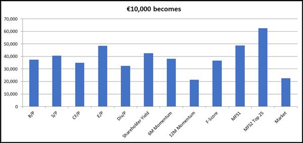
Before I get to all the details here are the summarised results:
Click image to enlarge
Here are the main points:
- There is a value premium in the European stock markets. This means value (undervalued companies) outperformed the market and glamour stocks (expensive or highly valued companies)
- Earnings / Price generated the highest return among the single-factor strategies
- Despite a lower geometric mean return of 10.9% Shareholder Yield had the highest Sortino ratio of 0.77
- The annual average value premium compared to the market ranged from 3.8% to 5.9%
- The annual average value stock premium compared to the glamour stock deciles (value companies did better than glamour companies) ranged from 11% to 17%
- The value deciles of all the multi-factor strategies outperformed their respective glamour deciles
- These results confirmed that previous research studies (mainly US studies) that investing in undervalued companies also works in Europe
- Combining value and momentum (the best strategy) to find undervalued companies that are already recovering (share price moving up), is a successful tool you can use to separate winners from losers
- Reducing portfolio diversification to 25 companies can increase your returns.
Click here to get these strategies working in your portfolio NOW!
Why did he do the research?
I like asking this question to see if the researcher may have any bias that may influence his or her results.
For Andreas it was a requirement of his master’s degree which he wanted to finish (and get a job afterwards) so he had to write a good paper. It’s unlikely that he had a bias he wanted to prove.
What did he want to find out?
Andreas wanted to answer the following questions:
- Given that a lot of studies about the value premium only looked at the US stock market he wanted to find out if value strategies also outperformed in the European stock markets?
- What single- or multi-factor value investment strategies were successful over this period, that is, had better risk-return properties compared to glamour stocks (companies that are expensive or over-valued) and compared to the market?
- Can these strategies also be used by institutional investors or are the results only theoretically achievable?
To do this he analysed the performance of 11 quantitative value investing strategies in Europe over the 13 year period from July 2001 to July 2014.
Market performance - basically flat with a lot of volatility
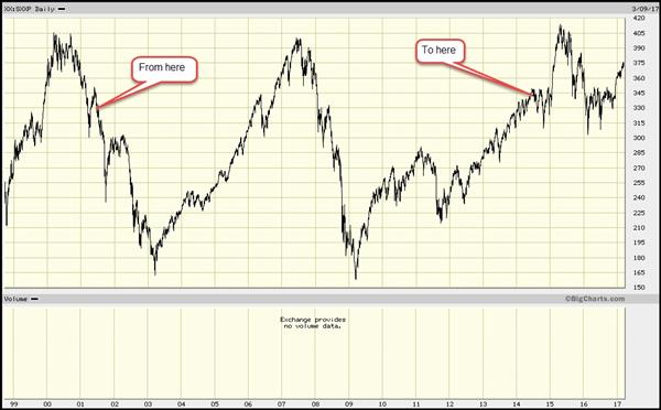
This is what the STOXX European 600 index did over the period of the research paper:
STOXX European 600 price index Source: bigcharts.marketwatch.com
As you can see it was a period with a LOT of volatility but the index did not go up much – it only went up about 3.6% over the 13 year period.
His “market” looked a lot different
The results of this research paper look a lot different because financial companies (which completely collapsed during the financial crisis) were excluded and dividends were reinvested.
In the paper the average return of the market over the 13 years was 7.5% and the geometric average 6.0%.
This means €10,000 invested in the market would have grown to €22,675 over the 13 years. Over the same 13 year period the maximum market drawdown was 55.9%.
What time period - Jul 2001 to June 2014
Andreas put the first portfolio together on 1 July 2001 and tested returns up till 30 June 2014. Portfolios were formed on a yearly basis (holding period one year).
Over the 13 year period he tested 11 investment strategies using 143 yearly portfolios.
The back test investment universe
He used the STOXX Europe 600 a stock market index instead of all the listed companies on the selected stock exchanges as the investment universe.
When he did the study the STOXX Europe 600 Index had a fixed number of 600 companies that represented large, mid and small market value companies from the following 18 European countries: Austria, Belgium, Czech Republic, Denmark, Finland, France, Germany, Greece, Ireland, Italy, Luxembourg, Netherlands, Norway, Portugal, Spain, Sweden, Switzerland and UK.
His reasons for choosing this index were:
- It covers 18 stock markets of developed European countries. Accounting for roughly 89% of the total market value of the European stock markets.
- The availability of index constituent’s lists allowed him to exclude survivorship bias (this is VERY important), as the exact composition of the index is known for the complete back test period. If he used only the current constituents’ list, as is common practice, it would have led to a survivorship bias, because returns from companies that were delisted during the back test period due to failure, acquisition or going private would not be taken into account
- The index allocation of 200 small, midsize, and large companies ensured an equal exposure to all sized companies and the back test is not dominated by large companies.
- To be eligible as for the STOXX Europe 600 index, a company must have a minimum average daily trading volume (ADTV) of USD 1.5 million, even for small companies. This is an important point to make sure all strategies can also be implemented in the real world, also by institutional investors.
-
Due to changes in the index during the back test period, 1141 companies were included in the index.
Companies excluded
Financial companies were excluded from the back test universe because their highly levered balance sheets distorted many ratios that were part of the analysis.
This reduced the universe over the back test period to 884 companies.
The data source
Fundamental and daily price data were obtained from Thomson Reuters Datastream.
In the case of different currencies than the Euro for fundamental data (UK companies for example), the accounting data was converted using the respective exchange rate of the day of portfolio formation.
All returns in Euro
Because Andreas aimed his research at European investors - all price and dividend data were converted to Euro.
The daily total returns were calculated for all companies in the investment universe in the period from 1 July 2001 until 30 June 2014.
Returns for companies that delisted were calculated based on their actual returns. These intra-year returns were only invested on the next date when portfolios were formed.
Portfolio construction
For the calculation of accounting ratios fundamentals are lagged by six months to prevent look-ahead bias.
This is done because companies release their financial reports several months after their financial year end. This approach is conservative as other researchers have lagged results only three or four months.
This means that, for companies with a December year end portfolios were only formed in July using December year-end financial data.
Invalid companies excluded
Companies with invalid ratios were excluded from the investment universe for that year.
Ratios were invalid if there was at least one missing data point or if the value did not pass certain plausibility criteria. For example, companies with negative book value, sales, dividends or market value.
Each year, for every investment strategy tested, decile portfolios and a benchmark portfolio was created.
The benchmark (market) portfolio consisted of all the companies for the respective year that had all the financial information available to implement the investment strategy. For example all the companies for which the book to price ratio could be calculated was included in the market return for the year.
This is important because it means the market for different strategies were not the same each year.
This may sound unusual but using a specific market portfolio for each year and investment strategy allows you to make accurate performance comparisons between all deciles of the investment strategy and the market.
It was also a good idea because the already small investment universe each year was not further reduced by the requirement to have valid accounting ratios for all the investment strategies for the year.
Click here to get these strategies working in your portfolio NOW!
Limitations of this back test
As with all back test studies there are a few things that you must always keep in mind and they are:
- The returns shown for the 13 years between 2000 and 2013 might not be representative in terms of risk and return characteristics for different time periods or stock market.
- The results are influenced by several simplifying or implicit assumptions. For example, reinvestment of dividends or the buying and selling of investments having no influence on prices.
- All returns are shown before buy and sell (bid and offer) spreads, transaction costs and taxes. This means, depending on your individual situation your returns may look a lot different.
Single factor strategies
- Book-to-Price (B/P) – this is the inverse of price to book http://www.quant-investing.com/blogs/general/2015/09/18/why-use-book-to-market-and-not-price-to-book
- Sales-to-Price (S/P)
- Operating Cash-flow-to-Price (C/P)
- Earnings-to-Price (E/P) – inverse of price to earnings
- Dividend-to-Price (Div/P)
- Shareholder Yield (Dividends + net share repurchase / Market value)
- 6-Month Momentum (Current share price / Share price 6 months ago)
- 12-Month Momentum (Current share price / Share price 12 months ago)
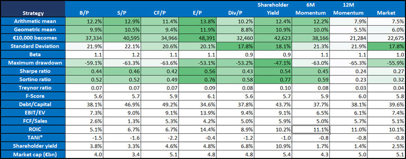
This was how the single factor strategies performed:
Click image to enlarge
The results:
- The two best performing strategies were E/P followed by Shareholder Yield
- Div/P was the strategy with the lowest volatility measured by standard deviation
- E/P and Div/P had the lowest maximum drawdown
- Shareholder Yield had the best risk adjusted returns as measured by the Sharpe and Sortino ratios
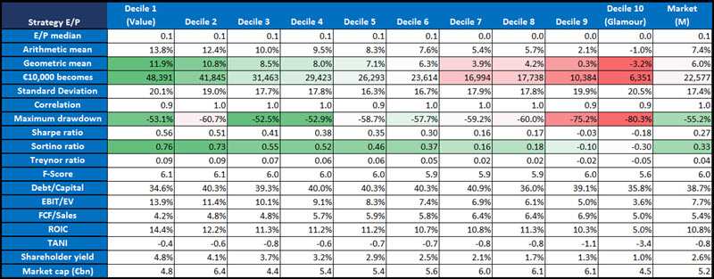
Best single ratio strategy - Earnings to Price strategy results
Click image to enlarge
*TANI = Total Accruals to Net Income = (Net Income - Operating Cashflow)/Net Income
Second best single ratio strategy - Shareholder Yield strategy results
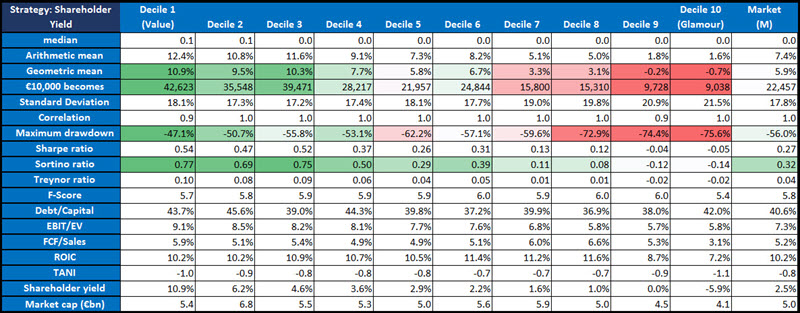
Click image to enlarge
Click here to get these strategies working in your portfolio NOW!
Multi-Factor Investment Strategies
- The F-Score strategy was the Piotroski F- Score combined with Book-to-Price. A good F-Score was defined as greater than 6 and a bad score less than 3. A bad Book to Price ratio was defined as smaller than 0.33 (Price to book ratio greater than 3) and a good book to price ratio as greater than 0.66 (Price to book ratio of smaller than 1.5)
- Multi-Factor Strategy 1 (MFS1) is similar to James O’Shaughnessy’s Value Composite Two which ranks all companies based on Book / Price, Earnings / Price, Sales / Price, EBITDA / EV, Operating Cash Flow / Price and Shareholder Yield. Instead of EBITDA / EV he used Div/P. He did this because he wanted this strategy to consist of all the single factor strategies he tested
- Multi-Factor Strategy 2 Top 25 (MFST2 Top 25) = Selected the 25 highest-scoring stocks per decile from the Multi-Factor Strategy 1 strategy but it also included 6-Month Momentum. It is thus a more concentrated strategy (only 25 positions) than the Multi-Factor Strategy 1 and it includes 6-Month momentum.
This was the performance of the multi-factor strategies:
Click image to enlarge
The results:
- The best strategy by far was Multi-Factor Strategy 2 Top 25 with Multi-Factor Strategy 1 (MFS1) in second place
- F-Score had the lowest maximum drawdown
- Multi-Factor Strategy 2 Top 25 also had the best risk adjusted returns measured by the Sharpe and Sortino ratios
Best multi ratio strategy - Multi-Factor Strategy 2 Top 25
First a reminder, the Multi-Factor Strategy 2 Top 25 (MFST2 Top 25) selected the 25 highest-scoring stocks per decile using the following ratios: Book / Price, Earnings / Price, Sales / Price, Div/P, Operating Cash Flow / Price and Shareholder Yield and 6-Month Momentum.
Here are the detailed results of the strategy:
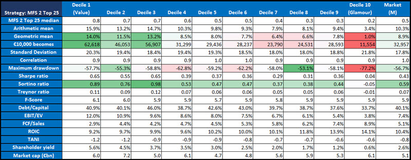
Click image to enlarge
Second best multi ratio strategy - Multi-Factor Strategy 1
Remember the Multi-Factor Strategy 1 (MFS1) is similar to James O’Shaughnessy’s Value Composite Two which ranks all companies based on Book / Price, Earnings / Price, Sales / Price, EBITDA / EV, Operating Cash Flow / Price and Shareholder Yield.
The difference between James O’Shaughnessy’s Value Composite Two and the MFS1 investment strategy is instead of EBITDA / EV he used Div/P.
It is a pity that this strategy was not also tested with momentum as I liked to see if Andres also found that momentum can add a lot to the returns as we found in our research study (also tested in Europe from June 1999 to June 2011).
Here are the detailed results of the strategy:
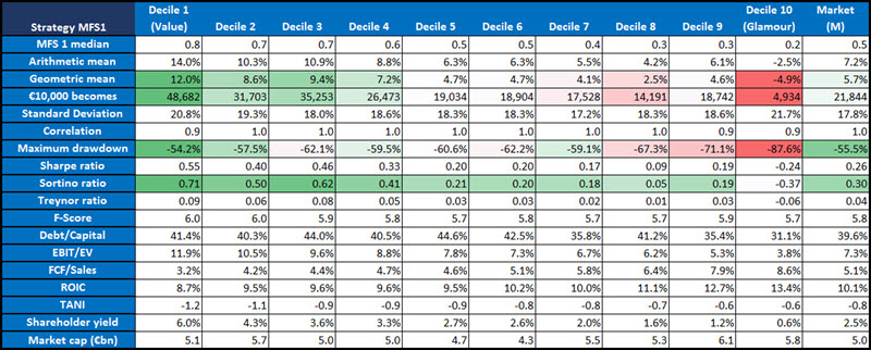
Click image to enlarge
Putting all the strategies together
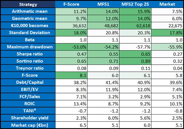
To help you make sense of all the results (single and multiple ratio strategies) I put them all together (only results of Quintile 1) in one table and added colour to the chart.
Red = bad or lowest value
Green = good or highest value

Click image to enlarge
The results:
- Multi-Factor Strategy 2 Top 25 was the best strategy
- 12m Momentum was the worse
- Div/P and F-Score has the lowest standard deviation
- Shareholder Yield had the lowest maximum drawdown and 12m momentum the highest
- Multi-Factor Strategy 2 Top 25 had the best risk adjusted returns and 12m momentum the worse
- Debt/Equity was quite low for all the strategies but there was no link to the best or worse performing strategies
- There was no link between ROIC and the strategies that performed best. This is something we also found in a lot of other research – quality as measured by ROIC does not help your returns.
Click here to get these strategies working in your portfolio NOW!
How implement the best strategy using the stock screener
To help you make use of the results of this research here is how you can easily find investment ideas using the best strategy from the paper.
How to implement the best strategy - Multi-Factor Strategy 2 Top 25
As I mentioned the Multi-Factor Strategy 2 consists of combining The Value Composite Two investment strategy with 6-months momentum.
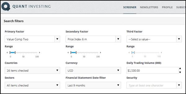
This is what you want to screen for:
- Select all the European stock markets – or the markets you want to invest in
- Select companies with a daily trading volume of at least $1.5 million (if you are a private investor you can lower this to the liquidity level you feel comfortable with)
- Select the 20% of companies with the best Value Composite Two ranking
- Select the 20% of companies with the best 6-months momentum
- Once you have a list of companies buy the 25 with the best Value Composite Two ranking
- You can either buy a few companies each month or as in the study buy 25 companies and re-balance your portfolio after a year
This is what the screen looks like:
Click image to enlarge
As you can see it is very easy to select the ratios and indicators you need which will give you a list of companies that look like this.
You can save this screen and export to Excel
You can save the screen – and open it with a few mouse clicks – making it easy for you to get the latest companies selected by the screen.
You can also export the companies selected by the screener to Excel to analyse the results further.
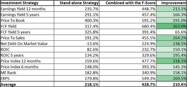
Improve these returns by an average of 200%
Some time ago we tested the Piotroski F-Score with 13 other investment strategies to see if it could increase the returns.
What we found was remarkable.
Combining the F-Score with another investment strategy can give you a lot higher returns – on average 210% over 13 years.
Here is a summary of by how much the F-Score increased the various investment strategies:
Click to enlarge
Here you can get all the information on how well the F-Score worked: Can the Piotroski F-Score also improve your investment strategy?
Even though we did not test the Value Composite Two with the F-Score, I am sure you will agree if it increased the return of 13 other investment strategies it is very likely to also increase the returns of the Value Composite Two investment strategy.
All this costs less than a lunch for two
How much can a tool like this to help you select market beating investment ideas cost, you may be thinking?
To make it affordable, and give you a great return on your investment, even if your portfolio is still small we have made the price of the screener very affordable.
It costs less than an inexpensive lunch for two each month (Click here for more information).
Don’t hesitate, you really have nothing to lose - if you are not 100% satisfied with the screener you get all your money back – guaranteed!
PS: Why not sign up now, while this is fresh in your mind?
Click here to get these strategies working in your portfolio NOW!


